| Calculating with Dates in Excel |
| Written by Janet Swift | ||||
| Tuesday, 05 January 2010 | ||||
Page 3 of 3
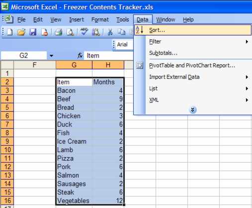
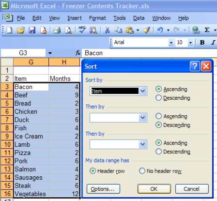
Using a look-up tableBefore we enter more data let's incorporate a look-up table of the storage times for food items so that we can use a formula to return the appropriate shelf life. Type in the headings "Item" (in G2) and "Months" (in H2) followed by a list of the items that you store in your freezer plus their corresponding maximum storage times in months. You can copy ours or devise your own. The important point to note is that having typed in the entries in two columns you need to sort them in alphabetically on the foodstuff's name. To do this select cells G2:H16, click on the Data menu and select Sort.
In the Sort dialog box we want select Item in the Sort by box and Ascending as the order. As we selected a range that includes headings ensure that Header Row is selected so that it is the range G3:H16 that is sorted.
Naming a rangeWhen using lookup tables it is a good idea to name the range that holds the table. To do this select G3:H16, drop down the Insert menu and select Name and Define.
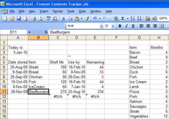
Now we can enter the lookup formula that returns the maximum storage period and as this is in months and we are working in days this has to be multiplied by 30, i.e. the formula to enter in C6 is =VLOOKUP(B6,Storage,2)*30. This looks for a match for "Steak" in B6 in the table and then returns the value from the second column of the table. Copy this formula and the ones in columns D and E down the column and don't worry about the #N/As that appear as we are now going to enter some more dates and food items. Extending the look-up tableI've used a bit of a cheat to produce the next 4 dates - I selected the existing two dates and extended the series with the fill handle. In column B I've entered Chicken (B8) followed by Fish (B9) and Ice Cream (B10) everything has worked nicely. However when I entered Beefburgers in C11 the shelf life is given as 270 which I know is far too long.
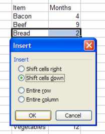
Type Beefburgers in the empty G5 and 2 in H5. As we have made an insertion in the middle of the look-up table the named range adjusts and now refers to G3:H20. If you add items above the top or below the bottom of the range remember to re-define the range name. For the final entry in this spreadsheet we will store something on the current date using the shortcut method of Ctrl+;. So in A12 use Ctrl+; - i.e. hold down the Ctrl key and press the semi-colon key (next to L) on the keyboard. This will result in today's date appearing in column A. Type "Pizza" into B12 and the formulas will provide the rest of the information. If you have created this spreadsheet remember to save it as Freezer Contents Tracker. If you just want to experiment you can download my version. Find more spreadsheets
|
||||
| Last Updated ( Friday, 07 August 2020 ) |

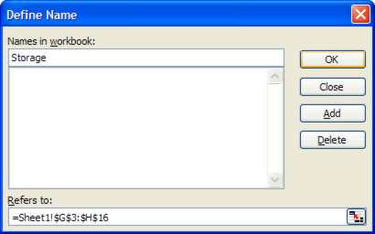
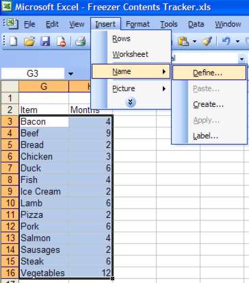 The Define Name dialog that appears suggests the first item in the list as the name. This isn't suitable so type in "Storage" and click OK. If you look at the range in the Refers to box you will notice the inclusion of dollar signs - a name ranged is automatically given an absolute reference and its position is fixed.