| Calculating with Dates in Excel |
| Written by Janet Swift | ||||
| Tuesday, 05 January 2010 | ||||
Page 2 of 3
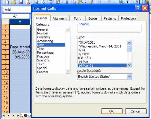
Date formattingThe way you type in a date isn't necessarily the way that it will appear. To see this in action now type 09-09-09 in A7 and notice that what appears in the cell is (probably) an alternative format. How dates display depends on the format being used and rather than leaving this to Excel it's a good idea to make a selection from the choices on offer. As we intend to use Column A for dates we will format the entire column. Right-click on the column heading, select Format Cells from the popup list, click on Date in the Number tab and then make a choice – here I've opted for using the month abbreviation as it makes it easy to read. After this however you enter dates in this column they will display in a consistent manner.
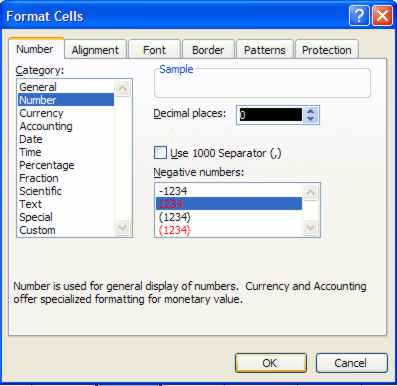
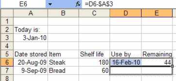
Enter "Steak" in B6 and its corresponding shelf life of 180 days in C6. To calculate its Use by date enter =A6+C6 in D6. You can do this by pointing - make D6 the active cell by clicking on it. Type =, click on A6, type + then click on A6 and press Enter. The answer should appear as a date formatted in your preferred style, i.e. 16-Feb-10. So far the dates that we have been working with have been fixed. A product stored on a given date needs to be used by another specific date to be safe. The time remaining before that date occurs, however, depends on the current date. This is something that "moves on" and needs to be updated every time the spreadsheet is opened. It therefore can be provided by the TODAY function which consults you computer's clock. Type "Today is:" into A2 and =TODAY() into A3. Notice that you need to start with = and finish with opening and closing brackets with nothing between them. What will appear in A3 when you initially do this is the current date. If you save the spreadsheet and open it again one or more days later the new date will show. To calculate the number of days remaining to eat an item stored in the freezer you need to subtract today's date from its Use by date. The formula to enter into E6 is =D6-A3 and the corresponding formula in E7 is =D7-A3. Notice that both formulae refer to A3 – so it needs to be specified as an absolute cell reference by the use of dollar signs so that it remains a fixed reference when the formula is copied down the column later on so we need to enter: =D6-$A$3 into E6. Pressing the F4 key once when entering or editing cell references adds the two $ signs to make a cell reference absolute. The answer you are expecting is a number but if instead you see the cell fill with ###s your spreadsheet has displayed the result of subtracting one date from another in date format and as there are no dates corresponding to negative numbers has resorted to hash symbols. To cure this problem we will format Column E to Number format available. So, right-click on the heading E, choose Format Cells and then click on Number in the Number section of the dialog box and set Decimal places to 0. At the same time you can select the red option for negative numbers.
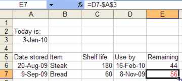
To see how this works type "Bread" into B7; 60 into C7 and copy the formulas in D6 and E6 into D7 and E7 by selecting the two cells and dragging down one row using the fill handle.
Notice that the number that appears in E6 is a negative number and is shown in red, indicating that the item has been stored too long.
|
||||
| Last Updated ( Friday, 07 August 2020 ) |