| Calculating with Dates in Excel |
| Written by Janet Swift | ||||
| Tuesday, 05 January 2010 | ||||
Page 1 of 3 Our freezer contents tracker puts the spreadsheet's date serial numbers to practical use. We look at date formatting and introduce a shortcut for entering and fixing the current date. 
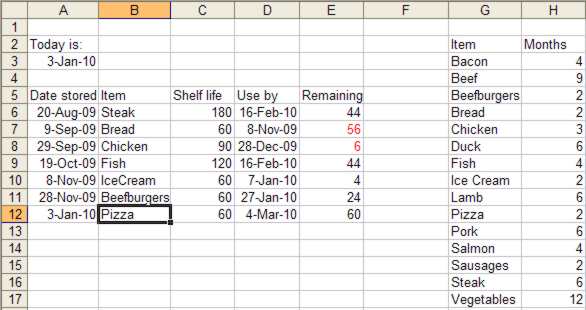
Date arithmetic using serial numbersDate arithmetic isn't straightforward. If you were asked exactly how many days you had already lived you would find it a pretty difficult task. Estimating it sounds trivial - multiply the number of completed years by 365 and then add the remaining days since your last birthday – but that would be an underestimate – you need to allow for leap years and the fact that there's no standard month length is an added complication. A spreadsheet can answer the same question in just three cells. Enter your birth date in A1, today's date in A2 and =A2-A1 in A3 to see the answer. In fact what you see probably won't answer your question until you deal with formatting issues. The spreadsheet method of answering questions about date arithmetic is a simple cheat based simply on counting. When you enter a date into a spreadsheet it converts it into a date serial number, numbering each day consecutively – starting at 1 and going up almost to 3 million - and when asked to do arithmetic with dates it's a simple matter of working with these numbers. This also explains the anomalous answer you'll have seen if you tried to discover your age in terms of days between two dates – as you are working with dates rather than showing you the difference in number of days it has treated it as another date serial number and displayed it as a date. To overcome this problem you need to format the cell to display a number and this is one of the aspects that our sample spreadsheet sets out to deal with. Excel supports two date numbering system. The default one the value assigns 1 to January 1st 1900 and 2958465 corresponds to December 31st 9999. The alternative one (provided for compatibility with early versions of Lotus 1-2-3) starts with 0, assigned to January 1st 1904 and goes up to 2957003 – the value for December 31st 9999. OpenOffice Calc offers both these systems for compatibility but its default has 0 corresponding to December 30th 1899. Unless you have a compelling reason stick with your spreadsheets' default date system but if you have to make a change you can do so in the Calculations tab of the Options dialog opened via the Tools menu. European and American datesExcel and OpenOffice calc are both very flexible in how they let you enter and view dates and give you plenty of options for customisation through formatting. One possible source of confusion is that different countries the interpretation of dates entered as numbers separated by oblique strokes differs. While mm/dd/yyyy is the standard American way to display dates in the UK and Europe dd/mm/yyyy is used. If when you type =TODAY() on January 4th 2010 and you see 01/04/10 or 1-April-10 when you choose the month abbreviation format the chances are you have the wrong international settings in force. To obtain the style you prefer go to Regional and International Settings in the Control Panel and ensure that you have the appropriate Regional Options in force. Date formatting is one of the aspects that our sample spreadsheet sets out to deal with along with short cuts for entering and fixing the current date. Dynamic and fixed datesAn obvious way to enter the current date is to use the functions TODAY and NOW. Dates entered this way update automatically – i.e. having saved the spreadsheet when you open it the next day, ten days later or a year hence the date you will see is the new current date. This is because these functions return the date and time supplied by the computer's clock. This is very useful but it poses a problem when what you wanted to enter is a fixed date. One possible method to "freeze" the date. That is having typed =TODAY() to enter the date convert it to a value by copying the cell (Ctrl-C) and using Edit, Paste Special and choosing Values from the pop-up dialog that appears. Excel offers a simpler way to enter the current data as a fixed value by using the shortcut Ctrl+; (i.e. hold down the Ctrl key and press ;). Freezer Contents TrackerAlthough our example is for a Freezer Contents Tracker the same idea could be applied to anything where shelf-life is an issue – film and photographic materials, chemicals, animal feedstuffs and so on.
To create your own version of this spreadsheet enter the title "Freezer Contents Tracker" in A1 and the following headings in Row 5: A5 Date stored To see how the spreadsheet works we'll start by listing some items that were stored last year. Although Excel stores dates as serial numbers (so internally it records August 20th 2009 as 40045) it lets you enter it in several more recognisable ways. It will recognise 08/20/09 or 20-Aug-09 as well as the full month name or abbreviation with or without dashes – so 20 August 09 works. Use the date format you prefer enter the date in A6. |
||||
| Last Updated ( Friday, 07 August 2020 ) |