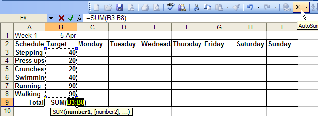
Summing totals

Next we'll add the formulas to sum the columns and rows.

The first column total to sum is for the Target minutes. Place the cursor in B9 and click on the AutoSum icon in the toolbar. Because there are numbers in the column above this empty cell Excel correctly deduces that we want to sum B3:B8 so press Enter to accept the formula =SUM(B3:B8).

(Click inside picture to expand it)

We now want to replicate the formula to cells C9 to I9. In other words we want to copy the same action but making it correspond to each new location, that is adjusting it to use relative cell references. We can do this using the same fill handle we have employed several times before. So put the cursor back into B9 and then drag the fill handle to the right ending in I9. When you let go of the mouse button C9 to I9 will fill with zeros.

The next task is to form the row totals for the minutes of exercise actually done and for this we need a new column with the label "Actual". It is usual to put the totals column at the right of the grid but there are two good reasons for putting it to the left:

1. If you use column J and then use AutoSum to will automatically include column B (Target minutes) and form the wrong sum.
2. For the purposes of the charts we are going to create later it will be very helpful to have Target and Actual in adjacent columns next to the activity names.

To insert the empty column place the cursor on the column label C at the top of the exisiting "Monday" column and right-click (click the right mouse button).  Click Insert on the pop-up menu that appears. The alternative method is to use Insert,Columns from the menu.

(Click inside picture to expand it)

You also need to type "Actual" into C1 - notice that it automatically appears in Bold.

We now need formulas to sum each of the totals for "Actual".  This cannot be done easily with the AutoSum icon which normally sums the entries to the left of the column. So place the cursor in C3 and type:

=SUM(D3:J3)

and press Enter.

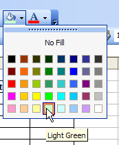
Then, using Autofill copy this formula to C4:C9.

Adding color shading

We are now going to apply some more formatting to make the Target and the Actual standout from one another, using two contrasting colors that we will use again when creating a chart.

Select B2:B9 and click on the down arror to the right of Fill Color icon in the Formatting toolbar and choose Light Green from the pallete of colors.

Repeat the operation with C2:C9 selected and choose light yellow.

Before entering any data into this grid copy the empty one together with an empty row for each of the successive weeks. The first such operation is to copy A2:J10 and insert the copied cells with the cursor in A12.

Now we are ready to transcribe the data for each of the weeks and the totals will be calculated automatically. Let's add the data for Week 1 and create a chart to show how well (or badly) it matched the orignal target.

(Click inside picture to expand it)

To save typing you can download Week1data.xls. If you want to copy it into your own worksheet select it all (Ctrl+A) and copy it into the next empty sheet, renaming it accordingly.

<ASIN:1419618474>

<ASIN: 0789736101>

<ASIN:0470044004>

<ASIN:0751338664>