Convert to a Function

Obviously we are going to need our conversion routine more than once so it makes sense to convert it into a function that returns a function that approximates the data. However there are a few small changed that are worth making. The first is that the plot is from 0 to n-1 which depends on the number of points in the data set. Much better to normalize it to be in the range 0 to 1 no matter what. The original data points at 0,1,2,3 and so on are now at k/n where k runs from 0 to n-1.

The second problem is that if you examine the function returned xp[t] you will find that it contains long decimal constants that look something like:

0.101036 Sin[3.28439 - 10 π t]

The examples in Wolfram Alpha have nice rational fractions in the formulas to make them look more hand crafted. Fortunately Mathematica has a Rationalize function which will convert decimal values into exact or approximate fractions. 

For example:

Rationalize[0.101036 Sin[3.28439-10 π t],
  0.001]

where the 0,001 specifies the accuracy of the approximation gives:

which looks a lot more friendly - no really, it does look easier!

So we need to modify the equation a little to produce a function that does the job:

trigSeries[x_] := (
 f = Chop[Fourier[x]];
 n = Length[x];
 hn = Ceiling[n/2];
 A0 = First[f];
 f = Take[f, {2, hn}];
 A = Abs[f];
 P = Arg[f];
 Function[t, Rationalize[A0/Sqrt[n] +
   2/Sqrt[n]*Total[A*Sin[Pi/2+
    2*Pi*Range[1, hn - 1]*t               
    + P]],
    .001]]
)

If you now try this out using the original data in x and y:

x = {0, 1, 4, 6, 8, 10, 8, 6, 4, 1, 0};
y = {0, 1, 1.5, 1.5, 1, 0,-1,-1.5,-1.5,-1,0};
xp := trigSeries[x];
yp := trigSeries[y];
ParametricPlot[{xp[t], yp[t]}, {t, 0, 1}]

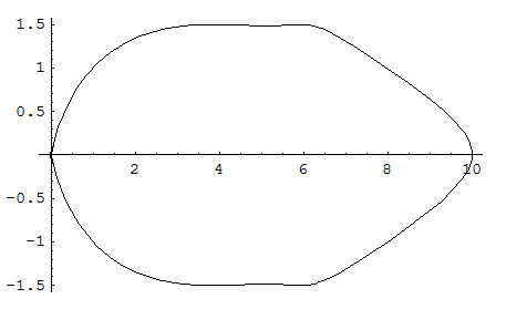
You will see a shape that looks a lot like the original but smoother. The reason for the smoothing is that the Fourier series is only an exact fit at the points x,y you specify. If you were to draw straight lines between these points you would have something that looks much more like the original:

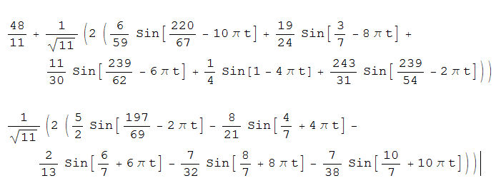
Notice the curve given above is created by plotting the two parametric formulas:

which look like the sorts of equations you can see listed in Wolfram Alpha and which would have taken a long time to find by trial and error or manual skill.  This may not be producing impressive graphics, but that is because what we started with wasn't impressive. Take a much bigger curve and digitize it to a set of co-ordinates and the same method will give you a pair of equations that approximate your original curve. From here it is only a short step to a portrait of Einstein - well it still quite a big step really.

Implementation in Python

The next trick is to implement the same idea in Python. You might initially think that this is impossible as Python isn't an math processing language like Mathematica. However we can do the same sort of trick by building up a string that has the same formula and then using the eval function.

You might also think that Python isn't ideal because it doesn't have a DFT function and not much in the way of plotting but these are easy to fix by importing MatPlotLib, Numpy and SciPy. 

So assuming we have these modules imported let's go though the steps to build up the formula and then put the whole thing together as function later. As a sort of exercise in Pythonic code no for loops were used or harmed in the development of this function. There are very definitely places were a for loop might have done the job more efficiently but...

First we need to perform a DFT and this is just a call to the SciPy fft  function:

import scipy as sp
import numpy as np
f=sp.fft(x)

The only problem is that SciPy uses a different definition of the DFT to Mathematica in that it doesn't use 1/sqrt(N) in the forward transform and uses 1/N in the inverse transform. These are the sort of minor differences that are sent to make numerical programming more difficult. The main point is that where we had 1/sqrt(N) in the formula we now need to use 1/N. 

Next we can extract the first term A0 from f:

n=len(x)
A0=abs(f[0])/n

Notice that we have already divided by n. In the case of Python it is easier to combine as many of the numerical values together as early as possible. 

Before moving on it would be a good idea to convert A0 into a fraction - i.e. as we did with Mathematica's Rationalize function. Python has a fractions module that can be used to find rational approximations. You need to add

from fractions import Fraction

and you can do the conversion using:

A0=Fraction(A0).limit_denominator(1000)

The final argument specifies the largest denominator that is allowed - the bigger the more accurate the approximation.  Notice that Fraction is a constructor for a fraction object and its methods.

Next we need to process the rest of the list f to get the other amplitudes and the phase angles:

hn=np.ceil(n/2)
f=f[1:hn]
A=2*abs(f)/n
P=sp.pi/2-sp.angle(f)

In this case we remove the first term from the first half of the list and then calculate 2^A/n and the Pi/2 minus the phase angle. Why are we now subtracting the phase angle rather than adding it? The SciPi angle method returns the phase angle computed from a different origin. Again these things are sent to make math programming difficult.