Repayment loans are the subject of the last of three chapters of Financial Functions with a Spreadsheet which look at the effects of regular cashflows.

 Financial Functions

 Buy from Amazon

Spreadsheets take the hard work out of calculations, but you still need to know how to do them. Financial Functions with a spreadsheet is all about understanding and reasoning, using a spreadsheet to do the actual calculation.

1. Understanding Percentages
   Percentages are something familiar to us all - but they present many pitfalls that need to be avoided.
   
   
2. Interest Simple and Compound
   We explore the idea of borrowing money for a specified rate of interest or earning interest on an investment. The ideas of Present and Future Value PV and FV are introduced. 
   
   
3. Effective Interest Rates
   We explore the idea of the `effective’ annual interest rate and then on to the Effective Interest Rate/Annual Percentage Rate, the much quoted EIR or APR.
   
   
4. Introduction to Cashflow - Savings Plans
   In the first of three chapters covering the way in which interest rate affects cashflow we explore savings - but first we introduce some general ideas that apply equally to annuities and repayment loans.
   
   
5. Cashflow Continued - Annuities
   We move on to annuities in the second of three chapters devoted to exploring the way in which interest rate affects 
   
   
6. Exploring Repayment Loans
   Repayment loans are the subject of the last of three chapters which look at the effects of regular cashflows.
   
   

7. Present and Future Values
   The principles of present and future value apply even if the cash flow is irregular. The calculations are just a matter of breaking down the cash flow calculations into simple steps.
   
   

8. Investment Analysis
   How is it possible to evaluate investments that generate irregular cashflows? We explore how NPV can be used to make investment decisions.
   
   

9. Advanced Investment Analysis IRR and MIRR
   The IRR is perhaps the most complicated of the measures of the value of an investment with an irregular cash flow. Understanding exactly what it means is a good step toward making correct use of it. 
   
   

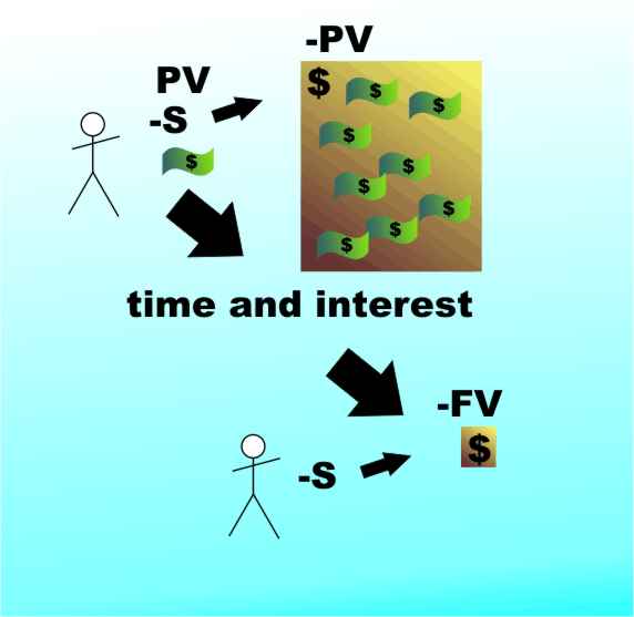
<ASIN:1871962013>

<ASIN:B07S79ZVMQ>

A repayment loan is particularly easy to deal with because it is just an annuity seen from a different point of view.

In the case of a repayment loan a sum of money - the principal or Present Value PV is borrowed at the start of the loan. At the end of each time period a regular sum S is paid back. This regular sum has to be large enough to pay back the interest due on the loan and some of the principal. As long as this is the case the proportion of interest to principal repaid each period changes so that more and more of the principal is repaid. Eventually the entire principal is repaid and the debt is cleared.

A repayment loan may be just an annuity seen from the other side of the table but the sort of questions you need to answer are subtly different. Partly this is due to a slight difference in psychology and the nature of the decisions you have to make. You are trying to minimize the interest rate and term rather than maximize them - but it is also the way that institutions and the law deal differently with loans than annuities.

In a repayment loan what interests us most is the size of the repayment given the loan, interest and term but there are still lots of reasons to need to calculate any of the four quantities - repayment, interest rate, term and loan amount - given the remaining three.

Turning the tables

The basic mathematics of repayment loans is the same as for an annuity. At the start of the loan the amount PV is borrowed - this is a cashflow in and so positive, however the balance in the account at this point is negative to signify a debt. 

At the end of the first period the debt has increased to:

PV*(1+I)

but the payment of S has also reduced it. That is, at the end of the first period the balance stands at:

PV*(1+I)-S

At the end of the second period the balance stands at:

[PV*(1+I)-S]*(1+I)-S = PV*(1+I)*(1+I)-S*(1+I)-S

and so on.

In general after n time periods the balance stands at

PV*(1+I)^n – S*(1+I)^(n-1)- S*(1+I) ...-S

which is of course the same as the situation encountered in the case of the ordinary annuity. Thus all of the equations, and even the spreadsheets. that we have constructed for the ordinary annuity apply to the repayment loan.

The only difference is that now the Present Value (PV) is the amount loaned and the payments are to repay the debt. After all one man’s annuity investment is another’s repayment loan.

In more practical terms this means that in terms of the cashflows the present value is positive because it is what the borrower receives, i.e. cash in, and the regular payments are negative, i.e. cash out. One final possible confusion is that the financial functions return a negative value of the PV or FV because it represents a debt.

Cash flow in a loan

The function:

=FV(I,nper,S,PV,type)

will calculate the Future Value FV of a repayment loan of PV being paid back at a rate of S per time period with interest at I%. As already explained type is 0 if the payment is at the start of the period and 1 if it is at the end.

For a repayment loan the payment is at the start of the period and isn't involved in the interest rate calculation until the following period. Also PV is positive and S (PMT in Excel's terminology) is negative.

In other words if you borrow PV at an interest rate of I% per period and pay the loan back at S per period then FV is the state of the account i.e. the debt after nper periods.

For example, if you borrow $1000 at 15% per annum paid annually then if you repay $200 per year after the first year the account stands at:

=FV(15%,1,-200,1000)

or -$950 i.e. the debt has reduced by $150. After 1 year the debt has increased to -$1150 and you have repaid $200 making a total of -$950 as given. In 10 years the debt is reduced to

=FV(15%,10,-200,1000)

which works out to $15.19 and a positive value indicates that the loan has been over paid by this amount - i.e. the loan was fully repaid sometime during the 10th year.

Number of periods to repay the loan

The FV function can be used to give the balance after any number of periods but it is also important to know when the loan is repaid - i.e. when the FV becomes zero.

To calculate the number of periods needed to reduce the Future Value to zero you can use the NPER function that has already been introduced in earlier chapters but this time with the FV set to zero:

n = NPER(I,S,PV,0,type)

For example, how long will it take to repay a loan of $1000 at 15% at a rate of $200 per year? The answer is:

=NPER(15%,-200,1000,0)

which works out to approximately 9.92 years. This agrees with the earlier calculation that the same loan is repaid before 10 years are up.