| Monthly Calendar |
| Written by Janet Swift | |||
| Monday, 14 December 2009 | |||
Page 1 of 2 This spreadsheet produces a versatile reusable calendar that can be printed out month by month

The DATE function used to be the one and only way to produce a date in a spreadsheet but given Excel's ability to recognise dates automatically its role has faded into obscurity. You have to be careful with syntax of the DATE function as it seems to be the wrong way round – you specify the year, then the month number and finally the day number. To see this in action open Excel and type in =DATE(1,2,3) – this produces the date 3-Feb-01. This hides another problem that only becomes apparent when you look at the date using a format that displays the year number in full. The cell contains the date 3 February 1901. So while you can drop the leading zeros in the month number and day number, don't take any short cuts with the year. However, if you leave the year out when entering dates Excel will automatically add the current year. Monday's childAnother Excel function, WEEKDAY, provides a quick way of discovering the day of the week of any date. To try out this function type the date 25-Dec into cell A3 in Excel and then in B3 enter =WEEKDAY(A3). You will see 6 appear there. That's not really what you want to see - it relies on you knowing that by default Excel counts from Sunday as 1 through to Saturday as 7. However, all you have to do if you don't want to convert from 6 to Friday for yourself is to use another useful function – TEXT – which converts from a date serial value to a specified number format. The format to give a full weekday name is "dddd" (or for a day abbreviation is "dd"). Try this out by entering or by entering =TEXT(A3, "dddd") in C3. There are also three functions that extract the day, month and year numbers from a date serial number. Again assuming that A3 contains the date 25-Dec, =DAY(A3) will return 25, =MONTH(A3) will return 12 and =YEAR(A3) will return 2009. A Calendar to InfinityOur example Excel spreadsheet, which you can download if you don't want start from scratch, makes uses of these functions to create a calendar display so that the user can specify any month of any year and instantly be shown it on a standard calendar grid. It also makes use of custom formats and in the final steps we add some cosmetic touches so that it can be printed out for use as a Month Planner, with or without a photo.
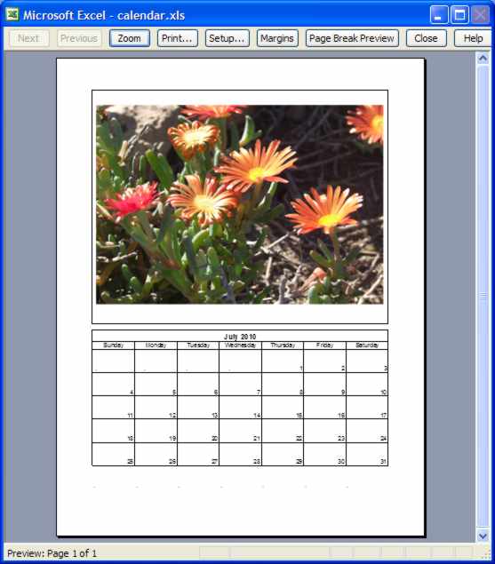
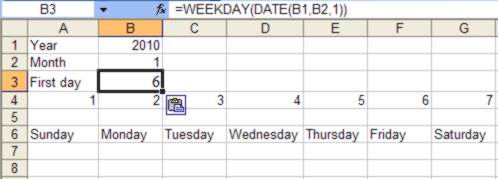
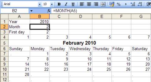
The finished calendar Although the idea of a month-to-a-view grid seems commonplace in fact it is a remarkably tricky problem since there is such an irregular correspondence between weekday and month days and yet you always want the grid to run from the beginning of the week – i.e. from Sunday to Saturday irrespective of the day on which the month begins. A month can have between 28 and 31 days and, depending on which day of the week the first of the month falls, can span a minimum of 4 and a maximum of 6 weeks. The clever part of our spreadsheet model is the formula that works out the parts of the grid that don't fall into the month we are interested in. Rather than leaving these cells completely empty we'll mark them with a discrete dot. This uses =IF, a function you are probably familiar with. We are also making use of the fact that while Excel stores dates internally as date serial numbers in the range 1 (corresponding to 1st January 1900) to 2958465 (corresponding to 31st December 9999). When you set the Number format of a cell containing a date to General you'll see the date serial number but using formatting you can a date in many different formats. First we'll create a calendar display with complete day names. Type Sunday into A6 and drag with the fill handle to G6 to enter the other day names automatically. For the purpose of the formula that places the days of the month in the correct position on the grid, we also need to enter the day numbers following the Excel convention that 1 equals Sunday, 2 equals Monday through to 7 for Saturday in Row 6. To save typing having entered 1 in A4 and 2 in B4 you can select these two cells and use the fill handle to extend this series to G4. Next we need a formula that works out the day of the week on which the month starts. To simplify this enter the labels "Year" in A1 and "Month" in A2 and "First day" in A3. Then type 2010 in B1 and 1 in B2 and enter the formula =WEEKDAY(DATE(B1,B2,1)) in B3. This returns the weekday number of the First day of the month specified in cell B2 in the year specified in B1:
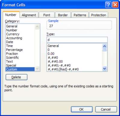
We can now use this day number to devise a formula to enter the day numbers on the first row of the calendar grid. The formula to enter in A7 is =DATE($B$1,$B$2,1+A4-$B$3). The first problem with this is the display – it shows the full date and we simply want the day number. To solve this we'll use a custom format to show the day number instead - but only after we entered all the formulas we need as they have the unwanted side effect of setting the formatting back to General. The second problem with the formula in Step 3 is that it results in dates from the previous month being included in the first row. To overcome this we need to check whether the date falls within the month specified in B2. If it does then we enter the day number and if not we place a dot in the cell. The formula that performs this uses an IF function and is entered in A7 as: =IF(MONTH(DATE($B$1,$B$2,1+A4-$B$3))=$B$2, Notice the use of absolute cell references here that allow us to copy this formula along the row to G7 still referring to the cells we are interested in. With the values of 2010 in B1 and 1 in B2 this formula results in dots in the first five cells then date serial numbers under Friday and Saturday. The day numbers for the second, third and fourth rows of the calendar grid can be produced by adding one to the previous day number. This can be done by entering two separate formulas then using the fill handle in each case to copy the formula to the other cells where it applies. The formula to add one to the day number of the first Saturday in the month to give the correct number for the Sunday in A8 is G7+1. Copy this to down the column to A9 and A10 using the fill handle. To go from Sunday to Monday through to Saturday in each row you refer to the cell to the left and add 1. So type A8+1 into B8 and use the fill handle to copy this five cells to the left and two rows down. The problem with using the same incremental method in the fifth and sixth weeks of the grid is that oat some point there will be a rollover into the following month. Again we need an IF function to discover whether to enter the day number or a dot into the cell and once this happens adding 1 to the previous cell results simply in #VALUE. To get around this we add 7 to the values in the fourth row of the grid to produce the fifth week's dates and, as there will often be dots rather than dates in this row we'll again rely on the values in the fourth row for the sixth row and in this case add 14 to them. Enter the formula: =IF(MONTH(A10+7)=$B$2,A10+7,".") into A11. This IF function checks whether cell A11 falls within the specified month and if so enters the day number in the cell, otherwise it enters a dot. Similarly enter: =IF(MONTH(A10+14)=$B$2,A10+14,".") into A12. Then use the fill handle to copy A11:A12 to B11:G12. Now for the formatting, select the range A7:G12, click the right-mouse button and choose Format Cells from the context menu. Click on Custom at the bottom of the Number tab of the dialog box and type d into the Type box:
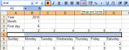
As soon as you click the OK button you will see day numbers replace all the date serial numbers. At the moment we expect the user of the calendar to type in two items of information – a year number and a month number. A couple of changes allows the user to enter month name and year as a single entry and have this displayed as the heading to the grid. Month names vary from three letters (May) to nine letters (September). To ensure the correct placement we'll merge the cells A5 to G5 and centre the text string within them. Select A5 to G5 and click on the Merge and Center icon in the Formatting Toolbar. You may need to open this toolbar using the menu item View Toolbars and placing a tick against Formatting.
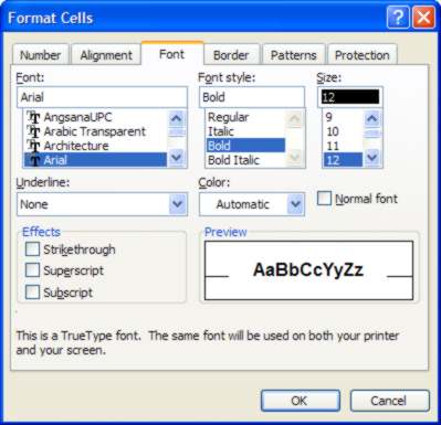
To make the month and year display as required needs another Custom format. Open the Format Cells dialog box again. You should find that Custom is already selected in the Category section in the Number Tab. Enter "mmmm yyyy" into the Type box. The click on the Font tab and choose the Font, here Arial, Font style, here Bold, and Font Size (here 12) that you require:
Now place the cursor within the merged cell in row 5 and type the date of Valentine's day using your preferred date format - 02/14/10 (for mm/dd/yy format in the US or 14/02/10 for dd/mm/yy which was used here). Although you will see the specific date in the Entry line you will see February 2004 appear over the middle of the grid:
We now need to enter formulae into B1 and B2, replacing the existing contents so that they use the entry in cell A5 as the basis for the calendar. Enter =YEAR(A5) into B1 and =MONTH(A5) into B2 and notice how the grid updates. The final steps are all cosmetic and are in preparation for printing the grid to a page for use as a month planner. Before continuing Save the spreadsheet under the name Calendar.xls. You'll can download this file if you want to start at this point.
Calendar.xls
|
|||
| Last Updated ( Friday, 16 April 2010 ) |