| The Ultimate Guide to Pivot Tables for Beginners |
| Written by Hannah Sharon | ||||
| Monday, 15 July 2019 | ||||
Page 2 of 3
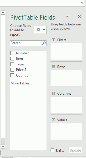
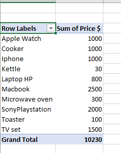
Step 4: Get to workOnce you’ve created your Pivot Table, figure out which fields you’d like to add or which ones you feel aren’t worth keeping. Each field is basically a column header from the source spreadsheet. In the Pivot Table Field, tick the boxes for each field you want to add. The chosen fields will be added to one of the areas below the Field List. Alternatively, you may drag a field to the needed area and the Pivot Table will calculate the selected fields. In our sample, we would like to get the total profit of all the goods sold. So we choose Item and move it to Rows and Price – move it to Values. Voila – you get Sum of Price and a neat table:
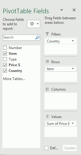
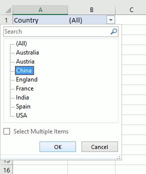
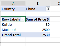
Sort, sort, sort Just like with any regular spreadsheet, you can sort the data in a Pivot Table using the Filter that can be found in the Pivot Table Fields. We could drag Country to Filters, and check how it affects our table. We get Country selection on the very top of the table where we can choose any country, let's say China, and check what goods were shipped to that destination.
|
||||
| Last Updated ( Monday, 15 July 2019 ) |

