| Evaluating an annuity |
| Written by Janet Swift | ||||
| Friday, 05 March 2010 | ||||
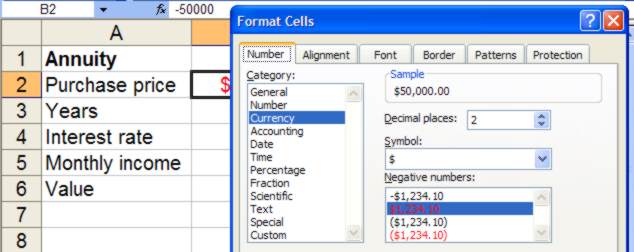
Page 1 of 3 In this spreadsheet we use Excel's financial functions and the Scenario Manager to help decide whether it is worth purchasing an annuity. In order to work with Excel's financial functions we also need to understand some terminology and conventions. Present Value, PV, is used for the sum of money involved at the start of a loan or investment and Future Value, or FV, for the final amount. In other words, FV is what results after interest (which is a percentage rate - so many percent per month, so many percent per year and so on) has acted on PV. By convention cash paid out is negative and cash paid in is positive. So in the case of an investment the cashflow out is negative but its future value is positive. For a fuller discussion of this see Chapter Four of Financial Functions. Annuity cashflowThe first function involved here is PV – the present value of a total series of future payments. The present value of a cashflow is simply the amount of money you would have to invest now at a prevailing safe interest rate to give you the same total amount of money as the total of the cash flow plus the interest it earns at the same rate. Enter titles and labels into a spreadsheet as follows: A1 Annuity A2 Purchase price A3 Years A4 Interest rate A5 Monthly income The annuity in our example costs $50,000 so enter -50000 in B2 – notice that it has to be negative because it is cash you are paying out. How this appears depends on formatting. Right-click on the cell B2 to open the Format Cells dialog, Choose Currency in the Number tab and then make a section in the Negative numbers section. Here we've selected the second option where negative numbers are shown in red.
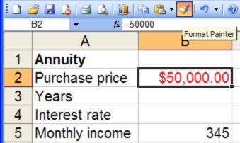
The annuity will pay the holder (money coming in) $345 per month so enter 345 in B5. Again set it to display in the same Currency formatting - you can easily do this by putting the cursor in the cell already set to this format and clicking on the Format Painter in the tool bar.
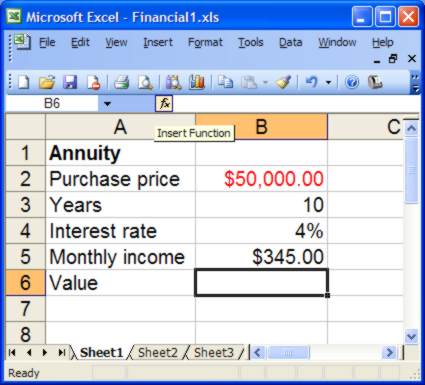
This "picks up" the format and you can "brush it" over cell B5. Notice that as a positive value it displays in black. Enter 10 as an initial value of years in B3 and 3.5% in B4 as the rate of interest. If you see 4% you' need to format this cell to display 1 decimal place, see the Loan Repayment spreadsheet if you are unsure about this. Using Insert FunctionNow we need to calculate the value of the investment using one of Excel's functions. When using a function you are unfamiliar with Excel's Insert Function facility is a great help. If you don't know which function you want to to use place the cursor in the empty cell and click on the fx button to the immediate left of the Entry line.
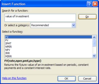
The search facility in the Insert Function dialog allows you to type in a brief description of what you require. In ths case you want to calculate "value of investment". Enter this is the top box and Excel selects FV - which is the required function, so click OK.
|
||||
| Last Updated ( Friday, 16 April 2010 ) |


