| How To Draw Einstein's Face Parametrically |
| Written by Mike James | |||||
| Thursday, 19 July 2018 | |||||
Page 2 of 4
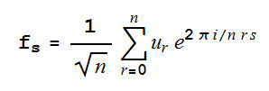
Using Discrete Fourier TransformOur next problem is to convert the coordinate sequence into a parametric function that generates the same sequence. The simplest way of doing this is to use the Discrete Fourier Transform function that Mathematica and PySci provide to fit trigonometric series to the data. If you don't already know about Fourier series don't panic at the next section simply accept the formulae and follow the general reasoning - and then realize why you really do need to study some math! This part of the explanation is complicated because the DFT is complex - i.e. written in the form of a series using complex numbers. In Mathematica the function Fourier[list] converts the list of values into a list of the same length of complex numbers. The formula for the conversion is:
where u is the list of data points and f is the list of complex amplitudes for each frequency. The important part of the DFT is that you can go back from the amplitudes to the data using the inverse DFT:
The important part is that we can obtain f from the Fourier function and by putting those values into the inverse formula we can get the original u values. So what? This seems like going round in circles, which it sort of is in an obscure mathematical way - but the whole point is that the inverse DFT formula is hiding the fact that it can be turned into the trigonometric series we are looking for. As long as the series u is composed of real numbers then half of the DFT coefficients are redundant as for s>0
More importantly it means that the complex exponentials can be reduced to cos by merging pairs of terms. The details aren't difficult but the algebra is long and not really relevant to the discussion. The final result is:
Where A is the magnitude of f and phi is the phase angle. As the examples quoted in Wolfram Alpha use sin rather than cos we can use the usual relationship between Sin and Cos to get:
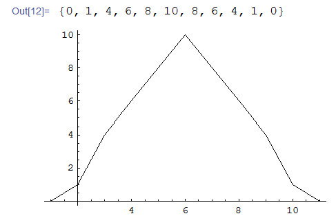
You can write the formula so the first term looks like the rest but be warned this can can produce problems when you try to find the phase of the first term if it is zero - i.e. if the original series has mean zero. Implementation in MathematicaNow we can implement the technique in Mathematica. The data can be the x co-ordinates from the "eye" plot:
Getting the Fourier coefficients, the f values, is easy:
and we only need the first half of the result and we need to remove the first term:
Now we can compute the magnitudes and the phase angles:
Putting all of this together we can now create a function that computes the original data using the previous formula for the sin series:
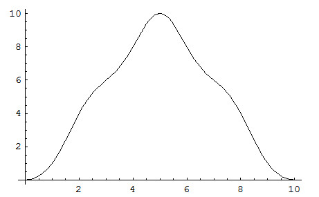
Now we have the function that approximates the original data. If you want to try it out you can evaluate xp[0], xp[1] and so on and discover that they are close to x[0], x[1] and so on. If you plot the function:
You might be surprised to find that the shape isn't exactly close to the original:
The point is that the approximation is only guaranteed to hold a the data points - between the data the series wiggles as a trigonometric series does. |
|||||
| Last Updated ( Friday, 20 July 2018 ) |


 Where * means complex conjugate. In other words the second half of the list of numbers is just the complex conjugate of the first half and this means we don't need them.


