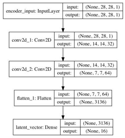
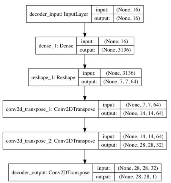
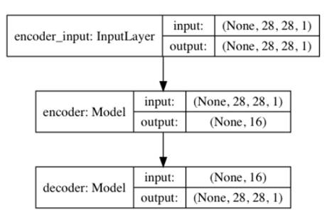
Figure 3: The encoder model is a made of Conv2D(32)-Conv2D(64)-Dense(16) to generate the low dimensional latent vector 

The decoder in Listing 3.2.1 decompresses the latent vector to recover the MNIST digit. The decoder input stage is a Dense layer that accepts the latent vector. The number of units is equal to the product of the saved Conv2D output dimensions from the encoder. This is done so we can easily resize the output of the Dense layer for Conv2DTranspose to finally recover the original MNIST image dimensions. The decoder is made of a stack of three Conv2DTranspose. In this case, we use a Transposed CNN (sometimes called deconvolution) which is more commonly used in decoders. We can imagine transposed CNN (Conv2DTranspose) as the reversed process of CNN. In a simple example, if CNN converts an image to feature maps, transposed CNN produces an image given feature maps. Figure 4 shows the decoder model. 

Figure 4: The decoder model is made of a Dense(16)-Conv2DTranspose(64) -Conv2DTranspose(32)-Conv2DTranspose(1). The input is the latent vector decoded to recover the original input. 

By joining the encoder and decoder together, we can build the autoencoder. Figure 5 illustrates the model diagram of the autoencoder. The tensor output of the encoder is the input to a decoder which generates the output of the autoencoder. We use MSE loss function and Adam optimizer. During training, the input is the same as the output, x_train. Note that in this example, there are only a few layers which are sufficient to drive the validation loss to 0.01 in one epoch. For more complex datasets, you may need deeper encoder and decoder and more epochs of training. 

Figure 5 The autoencoder model is built by joining an encoder model and a decoder model together. There are 178k parameters for this autoencoder. 

After training the autoencoder for 1 epoch with a validation loss of 0.01, we can verify if it can encode and decode MNIST data that it has not seen before. Figure 6 shows eight samples from test data and the corresponding decoded images. Except for minor blurring in the images, we can easily recognize that the autoencoder is able to recover the input with good quality. The results improve as we train for a larger number of epochs. 

Figure 6 Prediction of the autoencoder from the test data. First 2 rows are the original input test data. The last 2 rows are the predicted data. 

At this point, we may wonder how to visualize the latent vector in space. A simple method for visualization is to force the autoencoder to learn the MNIST digits features using a 2-dim latent vector. Then, we project this latent vector on 2D space to see how the MNIST codes are distributed. By setting latent_dim = 2 in autoencoder-mnist-3.2.1.py code and using plot_results() to plot the MNIST digit as a function of the 2-dim latent vector.

Summary

Autoencoders are neural networks that compress input data into low-dimensional codes in order to efficiently perform structural transformations. We demonstrated how to implement an autoencoder from two building block models, encoder and decoder. Extraction of hidden structure of input distribution is one of the common tasks in AI. Once the latent code has been uncovered, there are many structural operations that can be performed on the original input distribution. In order to gain a better understanding of the input distribution, the hidden structure in the form of the latent vector can be visualized using low-level embedding similar to what we did in this chapter or through more sophisticated dimensionality reduction techniques such t-SNE or PCA.

• This article is an excerpt from the upcoming book, Advanced Deep Learning with Keras, by Rowel Atienza and published by Packt Publishing. The core of the book focuses on the most recent successes of GANs and teaches developers to implement newer results for themselves, warning them of pitfalls and showing them the advantages of each.
  
  Use the code ORIPA09 at checkout to get recommended eBook retail price for $9 (valid till 15th Sept,2018)

To be informed about new articles on I Programmer, sign up for our weekly newsletter, subscribe to the RSS feed and follow us on Twitter, Facebook or Linkedin.

Related Articles

Reading Your Way Into Big Data