
| Autoencoders In Keras |
| Written by Rowel Atienza | ||||
| Monday, 03 September 2018 | ||||
Page 1 of 3 Keras enables deep learning developers to access the full power of TensorFlow on the one hand, while concentrating on building applications on the other. Even more surprising is its ability to write applications drawing from the power of new algorithms, without actually having to implement all the algorithms, since they are already available. .
This is an excerpt from the book, Advanced Deep Learning with Keras, by Rowel Atienza and published by Packt Publishing. This book is a comprehensive guide to understanding and coding advanced deep learning algorithms with the most intuitive deep learning library in existence. Introducing autoencodersAn autoencoder is a neural network architecture that attempts to find a compressed representation of input data. The input data may be in the form of speech, text, image, or video. An autoencoder finds a representation or code in order to perform useful transformations on the input data. For example, in denoising autoencoders, a neural network attempts to find a code that can be used to transform noisy data into clean ones. The noisy data can be an audio recording with static noise which is then converted into clear sound. Autoencoders learn the code automatically from data alone without human labeling. As such, autoencoders can be classified under unsupervised learning algorithms. Similarly, the succeeding parts of this book on Generative Adversarial Network (GAN) and Variational Autoencoder (VAE) are unsupervised learning algorithms. This is in contrast to supervised learning algorithms in the previous chapters where human annotations are required. In its simplest form, an autoencoder learns the representation or code by trying to copy the input to output. However, an autoencoder is not simply copying input to output. Otherwise, the neural network will not be able to uncover the hidden structure in the input distribution. An autoencoder encodes the input distribution into a low-dimensional tensor (usually a vector) that approximates the hidden structure that is commonly called latent representation, code, or vector. This process constitutes the encoding part. The latent vector is decoded by the decoder part to recover the original input. Since the latent vector is a low-dimensional compressed representation of the input distribution, it should be expected that the output recovered by the decoder can only approximate the input. The dissimilarity between the input and the output is measured by a loss function. Autoencoders have practical applications either in its original form or as part of a more complex neural network. Given a low-dimensional latent vector, it can be efficiently processed to perform structural operations on the input data. Common operations are denoising, colorization, feature-level arithmetic, detection, tracking, segmentation, and so on. The goal of this article is to present:
Principles of autoencodersAn autoencoder has two operators:
The encoder transforms the input, x, into a low-dimensional latent vector, z = f(x). Since the latent vector is of low dimension, the encoder is forced to learn only the most important features of the input data. For example, in the case of MNIST digits, the important features to learn may include writing style, tilt angle, roundness of stroke, thickness, and so on. Essentially, these are the most important information needed to represent digits zero to nine. The decoder tries to recover the input from the latent vector, Although the latent vector has low dimension, it has sufficient size to allow the decoder to recover the input data. The goal of the decoder is to make A suitable loss function,
Where m is the output dimensions (for example, in MNIST Similar to other neural networks, the autoencoder tries to make this error or loss function as small as possible during training. Figure 1 shows the autoencoder. The encoder is a function that compresses the input, x, into a low-dimensional latent vector, z. The latent vector represents the important features of the input distribution. The decoder tries to recover the original input from the latent vector in the form of
Figure 1: Block diagram of an autoencoder
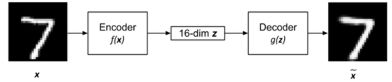
Figure 2: An autoencoder with MNIST digit input and output. To put the autoencoder in context, x can be a MNIST digit which has a dimension of 28 × 28 × 1 = 784. The encoder transforms the input into a low-dimensional z that can be a 16-dimension latent vector. The decoder attempts to recover the input in the form of Since both encoder and decoder are non-linear functions, we can use neural networks to implement both. For example, in the MNIST dataset, the autoencoder can be implemented by MLP or CNN. The autoencoder can be trained by minimizing the loss function through backpropagation. Similar to other neural networks, the only requirement is that the loss function must be differentiable. If we treat the input as a distribution, we can interpret the encoder as an encoder of distribution,
The loss function simply means that we would like to maximize the chances of recovering the input distribution given the latent vector distribution. If the decoder output distribution is assumed to be Gaussian, the loss function boils down to MSE since:
where |
||||
| Last Updated ( Sunday, 19 May 2019 ) |
 .
. as close as possible to x. Generally, both encoder and decoder are non-linear functions. The dimension of z is a measure of the number of salient features it can represent. The dimension is usually much smaller than the input dimensions for efficiency and in order to constrain the latent code to learn only the most salient properties of the input distribution. The autoencoder has the tendency to memorize the input when the dimension of the latent code is much bigger than x.
 , is a measure of how dissimilar the input, x, from the output which is the recovered input,
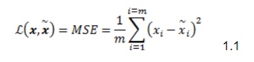
 and
and  are the elements of x and
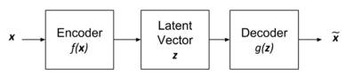
 and the decoder as the decoder of distribution,
  . The loss function of the autoencoder is expressed as:
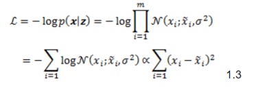
 is a Gaussian distribution with mean
  and variance of
  . A constant variance is assumed. The decoder output