| The Programmer's Guide to Chaos |
| Written by Mike James | ||||
| Thursday, 14 May 2020 | ||||
Page 2 of 3
Equilibrium and AttractorsEquilibrium is all about stability and chaos is the negation of stability. Classical science also concentrated on stability and systems in equilibrium and so chaos was a hard pill to swallow. It took a long time for a theory of chaos to emerge and some say that it is still emerging! The key idea was the generalization of equilibrium to “attractors”. Consider for a moment a simple pendulum. If you displace it and let it go then the pendulum will swing back and forth until it slowly but, and this is the important word, surely, runs down and returns to rest again. The equilibrium point where the pendulum comes to rest is called an “attractor” in the dynamics of the pendulum. In a “dissipative” system like the pendulum, i.e one that runs down, any displacement from an attractor always sees the system eventually return to another attractor. In a “conservative” system, i.e. one that doesn’t run down, then periodic behaviour is possible. For example, a pendulum driven by a clockwork escapement continues to swing backwards and forwards for as long as the spring has some energy. The earth continues to spin its way around the sun and so on. These periodic behaviours are also equilibrium or stable states and as such we can call them “attractors”. If you give the pendulum an extra push then after a while it returns to its original way of swinging. The attractor in this case is a set of points in space. To be more exact the attractor is a set of points in “phase space” – plot of position and velocity. A periodic attractor is a natural generalization of the idea of a simple point attractor which is a generalization of equilibrium. 
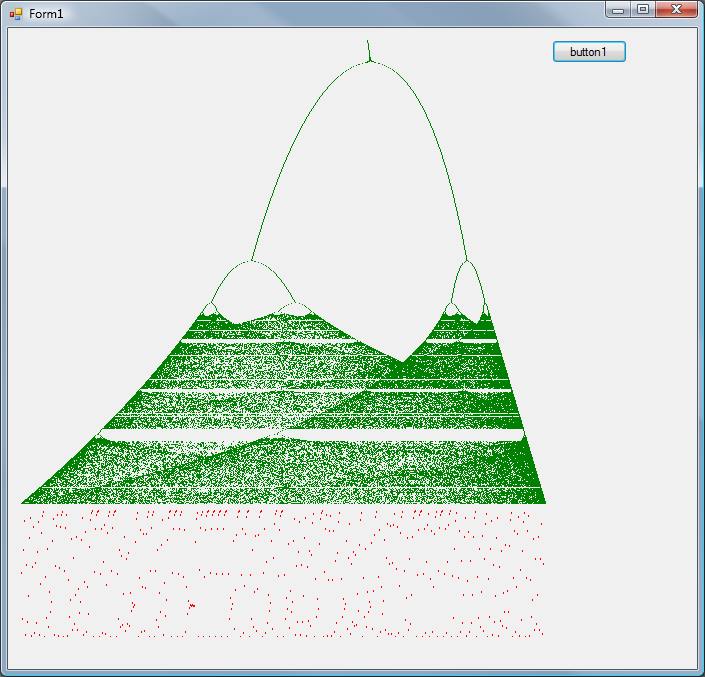
Non-linear systemsSo far we have just been talking about classical dynamics plus some more advanced 20th century ideas. Where chaos really comes into the picture, so much so that it cannot be ignored, is when we start to look at “non-linear” systems – that is systems governed by equations that involve powers of x, sin, cosine and so on, i.e. all but the very simplest systems. Sometimes non-linear systems do behave like simple linear systems in that they have attractors that are simple geometric shapes. This means that their behaviour is periodic, sometimes in complex ways but still essentially regular.The behaviour is still characterized by a sort of "equilibrium" state. However as we vary the parameters such systems sometimes change their behaviour for no apparent reason from this predictable regularity to something much more complicated and unpredictable and this we call the onset of chaos. Too much theory! So now an example. The Logistic MapConsider the simple equation: x <- ax(1-x) which means take a value of x, multiply by a constant a and by 1-x and this is your new value. This is called the logistic map and you can see that even though it isn't written in a way that makes it obvious this is a quadratic in x. that is it can be written as x <- ax-ax2 Clearly the logistic map is a non-linear system as it involves a power of x. Applying the logistic map once generates a new x value. Repeat this and you generate a sequence of x values. This iteration is a dissipative system like the pendulum and you need to run it for a while until it settles down and then see what patterns emerge.The value of a governs the amount of dissipation in the system and so we are interested in how the system behaves for different values of a. For values of a less than 3 the results are simple but for values between 3 and 4 the result degenerates into chaos. This can be seen in a “bifurcation” diagram created by plotting all of the x values that are turned up by the iteration after the system has settled down. To plot a bifurcation diagram you start the system off from an arbitrary initial x value and iterate for a while to let the system "forget" its starting point. Next you run the system and plot all of the x values that turn up in a line. You repeat this for a range of a values building up a plot as you go. For values of a less than 3 there is a single point attractor. As the value of a increases the single point splits into two and the system oscillates between these two attractors.This corresponds to the first part of the diagram with two branches. Then it splits again, and again and again until there are so many attractors that there is no obvious pattern in the behaviour. This splitting of attractors is called bifurcation and it is a common feature of the onset of chaos. At a value of a equal to about 3.56 the number of attractors becomes a fractal set and it is known as a “strange attractor”. At this point we have fully chaotic behaviour. Strange attractors are fractal attractor sets and they correspond to chaotic behaviour.
As the value of a changes the number of points in the attractor set doubles
<ASIN:0631232516> <ASIN:0387202293> |
||||
| Last Updated ( Wednesday, 13 April 2022 ) |