| QuickSort Exposed |
| Written by Mike James | |||||
| Thursday, 24 June 2021 | |||||
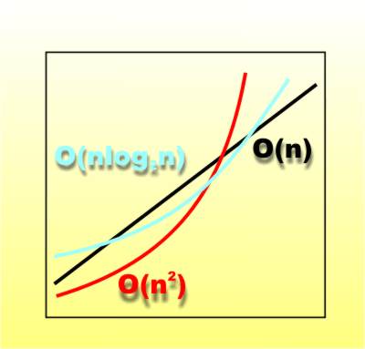
Page 1 of 4 QuickSort was published in July 1961 and so is celebrating its 60th birthday. QuickSort is the most elegant of algorithms and every programmer should study it. It is also subtle and this often means it is incorrectly implemented and incorrectly explained. Let's find out how it works and how to get it right. While I have programmed the QuickSort (QS) algorithm a number of times in different environments and explained it even more times, I have never been happy with either my understanding or my explanation of this most beautiful of all algorithms. Why do I say that it is beautiful? Well there are other algorithms that use similar strategies and achieve even more impressive results but there are none that relate to such simple matters. Anyone can understand the problem that QS solves and at each stage of its development there are no clever tricks or technical barriers to its understanding. And yet it is often difficult to see how this apparently simple algorithm works. As the QS algorithm is part of many an academic syllabus it is vitally important that it is well understood, even if you don’t actually want to use it at the moment! So let’s start at the beginning and work through to a completed program with nothing missing and no cover ups! O for OrderThe first thing to say is that there is a class of algorithm which use the same technique to speed things up. Let’s suppose we can create a straightforward algorithm that takes O(n2) operations say – O(n2) simply means that as the number of items involved in the algorithm, n, increases the amount of work the algorithm does goes up according to the square of n. Obviously we would prefer to use an algorithm that worked O(n) to one that worked O(n2) or even worse O(n3).
Orders of computation
Notice that this notation and ordering of the quality of algorithms is only a “long run” evaluation. For small n an O(n3) algorithm might well work faster than an O(n) algorithm. All we are assured of is that if n is large and getting larger sooner or later an O(n) algorithm will be faster, much faster than an O(n3) algorithm. Divide and conquerGoing back to our O(n2) algorithm for a moment there is a general strategy that can be used to speed it up. Suppose for a moment that we can find a way to split the list of things that we want to work on into two equal halves, each n/2 in size. If we can apply the existing algorithm to the first half and then to the second half we have an new algorithm that runs in O((n/2)2) + O((n/2)2) which if you work it out is actually faster than O(n2) by a little. If you can gain a speed up by dividing the list in half once why not do it again? You end up with having to operate on a list of size n/4, n/8 and so on until you get down to a list size that consists of only one or two members which is trivial to work on. What usually happens is that each division takes n operations and there are log2(n) of them (log2 = log to the base 2). In this way the whole algorithm only takes O(n log2n) which for largish n is very much faster than O(n2) but still slower than O(n). This all sounds wonderful and indeed this approach - often referred to as "the divide and conquer" method - has given us many “fast” algorithms but there are a number of conditions that have to be satisfied. The main one is that the division of the list into two n/2 lists has to be such that the operation can be performed on the two halves independently. In other words there is no use in splitting the work into two halves if you still have to operate between the halves to complete the algorithm – this is no split! The split has to be real! Also the work involved in doing the split has to be small enough to produce a gain in speed. There is no point in doing an incredibly complicated split operation that takes O(n3) compared to a basic O(n2) algorithm because then you end up with a “quick” algorithm that works O(n3 log2 n), which is worse than O(n2). All of this reasoning has been very rough and far from precise but it's the way to think about everything before you make an attempt at making things precise. Now let's turn our attention to a very specific application of the divide and conquer principle - the quick sort. If you would like to see another application of the idea then have a look at Quick Median. The Postman's SortBefore we move on it is worth asking the question - how quickly can we sort. It is often thought that it takes an algorithm that scales like O(n2) to perform a simple sort or if you are being clever then perhaps you can get this down to O(n log2n) but in fact sorting can be performed in O(n). This algorithm is called the Postman's Sort because it is close to the system used to sort mail. Suppose you have a set of five numbers between 1 and 10 and you need to sort them. First create an array with ten elments and scan through the list and do:
In other words, put the item with the value v in the array element array[v]. This produces a perfect sorting in just one pass through the data and so it is O(n). The problem with the Postman's Sort is that it needs one array element for each possible data item. For example, try sorting five values in the range 1 to 5 million. Now you need an array with 5 million elements which doesn't look so attractive. Practical versions of the postman's sort make use of hash functions to condense the range of possible values that can occur however hash functions are another story.
<ASIN:0763707821> <ASIN:0201896850> <ASIN:0817647287> <ASIN:059651624X> |
|||||
| Last Updated ( Thursday, 24 June 2021 ) |