| The Monte Carlo Method |
| Written by Mike James | ||||
| Thursday, 27 July 2017 | ||||
Page 2 of 3
Generating Any DistributionThe way that you do this is to use the inverse cumulative probability function F-1(p) which gives you a value x that satisfies F(x)=p i.e. the probability of getting x or less is p. What you do to generate random values with the distribution F(x) is generate a random number r in the range 0 to 1 and return F-1(r). If you think about this graphically then you can see that the areas that correspond to each value x generated are proportional to the probability of x. For example, in the case of the dice example if the random number r generated is between 4/6 and 5/6 then F-1(r) is taken to be 5. You can see that the areas are divided up equally to generate values with a probability of 1/6th.
In general the areas don't need to be divided equally and the cumulative probability function can be continuous. The algorithm works in a very regular way for any distribution:
Usually the cumulative probability function is available as an approximate table of probabilities and the inverse function can be created by simply using the table "the other way round" i.e. by looking up the probability and returning the value. The Monte Carlo methodAfter looking at some of the ways that you can manipulate random numbers it is time to return to our main subject – the Monte Carlo method. It isn’t difficult to think up serious uses of random numbers in a computer. For example, to find out how many pumps were needed at a petrol station you might simulate the situation. All you would need to do is write a program that allowed cars to join queues at the pumps with the correct statistical distribution and rate. You would also have to make sure that each fill of the tank took an appropriate amount of time and all the other random delays were included in the model. At the end of the simulation the program would provide you with a figure for the average queue length. Notice that a simulation doesn’t give you the exact answer fixed and unchanging. It’s just an estimate of the answer and if you run the simulation again you will get a different answer. In practice of course you can put a probability estimate that places the answer in a given range with a high probability. For example, the queue might be estimated at between 8 and 11 with 90% certainty. Which means that in 90% of the simulations you ran this is what the queue length was between. If you think too deeply about this you can start to get worried. After all if there is a 90% chance that it is in this range but there is a 10% chance that it is outside of this range! In fact there is a probability that it is any value you care to think of! Of course in practice you don’t get worried because after throwing a coin 100 times and finding that the estimate of it coming down heads is around 0.5 you are very happy to accept this as a reliable estimate of the value. Simulations are somehow an “obvious” use of randomness to work something out, but it can get a little stranger than this because some problems that seem to have nothing to do with randomness can be solved by converting them into a form that can be simulated. Mostly when you think about working out problems using a computer you think of writing a program to solve something exactly. For example, if you want to find the area of an irregular shape then the usual way of doing this is to divide the shape up into small rectangles, work out the area of each one and add the whole lot up. Of course the answer isn’t exact but if you make the rectangles smaller and smaller you get closer and closer to the correct answer.
The smaller the rectangles the more accurate the area
You may be wondering what this has to do with random numbers? The answer is that this process of finding areas gets really tedious when you start to extend it to finding volumes and their higher dimensional counterparts. Finding areas, or integrating functions, is a very important tool in physics and engineering and it was the area under a particular curve that was holding up the A bomb project. The computers of the day just couldn’t do the sums fast enough. Then John Von Neumann thought of a simpler way of doing the same job using random numbers. To see how this works just think about firing a gun randomly at a target. The number of times you actually hit the target is going to be proportional to the target’s size or area. This is all there is to the Monte Carlo method. For example, suppose we want to find the area of a circle. All we have to do is generate random (x,y) points and count the number that hit the circle and the number that don’t. If you do this enough times then the ratio slowly settles down to the ratio of the area of the circle to the background area. You might think that converting this perfectly deterministic calculation into a game of chance is a crazy idea but you have to remember that generating random pairs is cheap and so is testing for a hit. Compared to the computational difficulty of dividing the shape up into little strips it is a very cheap way to work out an area and what is more the pay off gets better as you increase the number of dimensions you are working with. This is the reason that the area under an important function in the atomic bomb problem was worked out using random numbers.

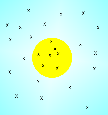
As easy as pie
Hitting the target – at random
OK, finding the area might not impress you but what about calculating one of the fundamental mathematical quantities using randomness. Pi is a well known target for programmers trying to make their name by computing it to a million more decimal places but what about making it a real target for a change. If you set up a circle with radius one then its area is exactly Pi and so finding the area using random numbers gives you an estimate of pie – I’m tempted to say as easy as… The idea of finding Pi using random numbers was invented in the eighteenth century by a French naturalist called Georges-Louis Leclerc, Comte de Buffon. He asked what was the probability of a needle thrown at random on a floor made up of planks with a width twice its length landing on a crack between planks. This very linear question has the answer 1/Pi and so you can count the number of times it lands on a crack and use this to estimate 1/Pi and by simple arithmetic Pi itself. It was actually tried out in 1901 and yielded 355/113,i.e it hit the crack 113 times in 355 throws, or 3.141592.. for the value of Pi which isn’t bad considering all they did was toss a needle onto the floor. Let's implement the algorithm in JavaScript. To make things easier we can place a circle with a radius 0.5 in the middle of the unit square. This circle has area 1/4 Pi and so counting the number of hits as a ratio of the total will estimate 1/4 Pi. <ASIN:0387212396> <ASIN:9812389350> <ASIN:0412055511> |
||||
| Last Updated ( Thursday, 14 March 2019 ) |